![]()
Analyze data
Follow this procedure to process your single molecule videos (SMVs) or trajectories and characterize the molecule dynamics in your sample.
Note: Skip step 1 if already in possession of intensity-time traces (ASCII files or in a mash project).
- Step 1: Create traces
- Step 2: Find states in traces
- Step 3: Identify state network
- Step 4: Determine state populations
<< PREVIOUS: Create traces NEXT: Identify state network >>
Step 2: Find states in traces
In this step, single molecules are sorted, intensity-time traces are corrected from experimental bias and state sequences are inferred for individual traces.
- Import trajectories
- Correct for experimental bias
- Sort time traces
- Discretize time-traces
- Save and export
- Merge projects
Import trajectories
Intensity-time trace correction, sorting and discretization is done with module Trace processing. Traces can be read from a MASH project created in Step 1 or from a set of ASCII files.
In the first case, you can skip this step and go to step 2.
To import trajectories from ASCII files:
-
Press
 in the
project management area; a window pops up:
in the
project management area; a window pops up: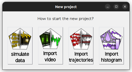
-
Select
import trajectoriesto open the experiment settings window and fill in the description of your experiment setup and the structure of your trajectory files; please refer to Set experiment settings for help -
Set the default export destination by pressing
 in the
project management area and selecting your root folder
in the
project management area and selecting your root folder -
Save modifications to a .mash file by pressing
 in the
project management area.
in the
project management area. -
Select module Trace processing by pressing
 in the main
tool bar
in the main
tool bar
Correct for experimental bias
Intensity-time traces must be corrected from experimental bias to obtain state trajectories that describe molecule dynamics the most accurately.
Experimental bias include shifts in molecule positions, background light and cross-talks between wavelength ranges used for emitter detection (bleedthrough) and excitation (direct excitation).
To adjust single molecule positions in panel Sub-images:
-
Select the shifted molecule in the Molecule list of Sample management
-
Select donor excitation in menu (a) of Single molecule images
-
Press
 in
Single molecule coordinates
in
Single molecule coordinates -
Go back to step 1 until all shifted molecules are recentered
To correct intensities from background light:
-
Define Background correction settings for each trace selected in menu (a):
default: method
<N median values>
default: option (h) activated and parameter (d) to 20 pixels -
Activate option Apply background correction for each trace selected in menu (a) of Background correction settings if not already done.
-
Press
 to apply the same settings to all molecules
To re-sample trajectories and increase SNR:
-
Set the Trajectory sampling time to a larger value:
default: Trajectory sampling time set to original video/trajectory sampling time
To correct intensities from cross-talks (if you are working with single detection channel and single laser illumination, ignore this step):
-
Set for each emitter selected in the Emitter list:
default: Bleedthrough coefficients set to 0
default: Direct excitation coefficients set to 0
Sort time traces
Now that molecule positions and intensities are corrected, we can reliably exclude irrelevant intensity-time traces from the project, e. g incorrectly labelled species, and sort relevant traces into subgroups.
To remove incorrectly labelled species from the project, the molecule has first to be identified and tagged. Then, Tagged molecules can be deselected and cleared from the project.
To tag species missing emitter label [E]:
-
Press
 in
Sample management to open the Trace manager
in
Sample management to open the Trace manager -
Select tool Overview
-
In Molecule selection, add the default tag
no-[E]by typing the tag name in (b) -
Select tool Automatic sorting
-
In panel Data, set menu (a) to
total [E] (at [W]nm), the total intensity of emitter[E]with[W]the emitter’s specific excitation wavelength, menu (f) tonone, and set parameters:default: option
original time tracesin menu (b)
default: parameters (c) and (d) to minimum and maximum intensities respectively
default: parameter (e) to 50 -
Define a range including the histogram peak centered on zero by clicking on the Histogram plot
-
In panel Range, set parameters:
defaut: option
at leastin menu (e)
defaut: parameter (f) to 90%
defaut: optionpercentage of the tracein menu (h) -
Select the option
total [E] (at [W]nm)in menu (a) of Concatenated trace plot and verify that selected traces are fluctuating around 0 -
Press
 in panel
Range to save range settings
in panel
Range to save range settings -
Select menu (b) to
no-[E]in Tags and press to assign this label to the selected range
 -
Press
 to tag with
 no-[E]all molecules missing emitter[E]
To clear species missing emitter [E] from the project:
-
Select tool Overview
-
In Molecule selection, select option
remove no-[E]in menu (a) to deselect all molecules carrying this tag -
Press
 in
Overall plots to close Trace manager and export the current selection to Trace processing
in
Overall plots to close Trace manager and export the current selection to Trace processing -
Press
 in
Sample management to delete deselected molecules from the project
in
Sample management to delete deselected molecules from the project
Discretize time-traces
To obtain reliable state trajectories, photobleached or interrupted data must be ignored and ratio-time traces must be corrected prior applying the state finding algorithm. This is done by splitting trajectories manually, automatically detecting and truncating the trace at dye photobleaching and setting/calculating global gamma and beta factors.
To split trajectories at intensity interruptions:
-
Define in Photobleaching:
default: method
Manual
default: parameter Photobleaching cutoff to the ending position of the interruption
default: optionCutdeactivated -
Press
 to separate the left- and right-side of the splitting position to separate trajectories
To truncate trajectories at photobleaching:
-
Define in Photobleaching:
default: method
Threshold
default: dataall intensities
default: parameters in Automatic detection settings (b) to 0, (c) to 2 frames and (d) to 10 frames
default: optionCutactivated -
Press
to apply the same settings to all molecules -
Press
 in
Sample management to process all molecules in the project and visualize truncated trajectories
in
Sample management to process all molecules in the project and visualize truncated trajectories
To automatically calculate gamma and beta factors (if you are working without FRET calculations, ignore this step):
-
For each FRET pair listed in the FRET pair list in Factor corrections, define:
default: method
ES linear regression(if you are working without stoichiometry calculations, use any other method)
default: in ES linear regression, (b) toAll molecules, (c) to -0.2, (d) to 50, (e) to 1.2, (f) to 1, (g) to 50, (h) to 3and press
 to calculate the ES histogram and perform linear regression, and
 to save settings
 -
Press
to apply the same settings to all molecules -
Press
in the
Control area to process all molecules in the project
To obtain state trajectories:
-
Define in Find states:
default: method
STaSI
default: apply toall
default: Method parameters (b) to 5 for each trace selected in menu (a)
default: no Post-processing methods with (b) an (c) set to 0 -
Press
to apply the same settings to all molecules -
Press
in the
Control area to process all molecules in the project
Save and export
Project modifications must be saved to the .mash file in order to perform Step 3 and Step 4 with processed data.
Beside, various ASCII and image files containing processed data, data statistics and processing parameters can be exported for use in other software.
To save project modifications:
- Press
in the
project management area and overwrite the current
.mash file or create another project file to keep a backup of unprocessed data
To export processed data to ASCII and image files:
-
Press
 in the
Control area to open and set export options; please refer to
Set export options for help
in the
Control area to open and set export options; please refer to
Set export options for help -
Press
 to start file export.
Merge projects
After applying proper corrections to intensities and sorting out molecules, samples from different projects with identical experiment settings can be merged into one big data set. This prevents to repeat the following data analysis procedure on multiple mash files and allows to constitute a more representative sample of molecules.
To merge projects:
-
Select the multiple projects to merge in the Project list
-
Right-click in the Project list, choose the option
Merge projectsand press to start the merging process
Note: The merging process induces a loss of single molecule videos that were used in individual projects. Make sure to perform all adjustments of molecule positions and background corrections prior merging.