Set experiment settings

Follow the appropriate procedure to set the experiment settings of your new project. To create a new project, please refer to First steps.

<< PREVIOUS: Video-based project NEXT: Histogram-based project >>

Option 3: Trajectory-based project

In this section, experiment settings are set for projects starting with trajectories import.

They are specific to each project and include video channel information, emitter and laser configurations, FRET and stoichiometry calculations, the structure of trajectory files but also experimental conditions and colors used to present data.

They are initially set when creating a new trajectory-based project by pressing New project in the
Project management area and can be edited by pressing Edit project in the same area.

Press Next to navigate through the settings and Save to complete the creation of the new project or immediately apply the modifications to the existing project.

Import
Channels
Lasers
Calculations
File structure
Divers

Import

Use this tab to define the trajectory and annexed files to be imported.

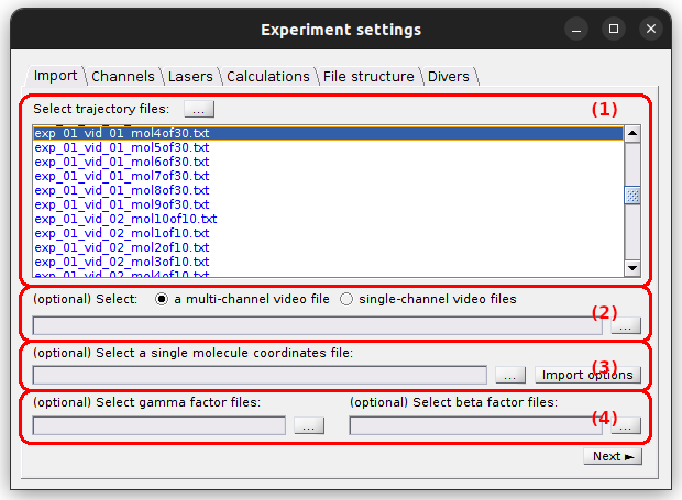
(1) Trajectory files
(2) Video file
(3) Coordinates file
(4) Correction factor files

Trajectory files

Imported intensities are used to build initial intensity-time traces and are therefore considered to be exempted of any correction. If intensities are already corrected of some sort, do not forget to deactivate the corresponding corrections in module Trace processing after import.

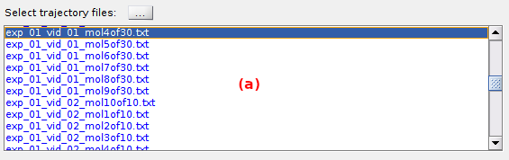
To import a set of trajectory files, press and select the files in the browser. Trajectory files are then listed in (a).

Trajectory files can contain data of one or multiple single molecules. Their structure must follow certain rules:

intensities specific to the emission channels must be organized in a column-wise manner,
intensities specific to laser illuminations can be organized in a column- or row-wise manner,
(optional) time stamps must be organized in a column-wise manner,
(optional) state sequences specific to the FRET pairs must be organized in a column-wise manner.

Video file

The single molecule video is used to recalculate initial intensity trajectories when the molecule position is modified, and in a specific background calculation. If no video is available, intensities will not be recalculated and only manual background setting will be allowed.

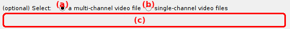
It is possible to import one multi-channel video (where a video frame is spacially divided into a number of emission channels) or multiple single-channel videos recorded in parallel (where each video contains a single emission channel) by activating the option (a) or (b), repsectively.

The interface (c) defines the video files to be imported and depends on the import type:

Import of a multi-channel video
Import of single-channel videos

default: multi-channel video.

After reading the necessary information from the video file, MASH calculates the channel- and laser-specific average images shown in tabs Channels and Lasers, respectively.

Calculate average image

Once the import is completed, the Video sampling time is automatically updated is tab Divers and the channel- and laser-specific average images in tabs Channels and Lasers, respectively.

Supported file formats are:

Olympus CellSense Format (*.vsi associated with *.ets)
Source Input Format (.sif)
WinSpec CCD Capture format (.spe)
Single data acquisition format (.pma)
Audio Video Interleave (.avi)
Tagged Image File format (.tif)
Graphics Interchange Format (.gif)
MASH video format (.sira)
Portable Network Graphics (.png)

New video formats can be added programmatically by updating the following functions in the source code:

MASH-FRET/source/mod_video_processing/graphic_files/getFrames.m
MASH-FRET/source/mod_video_processing/graphic_files/exportMovie.m

Import of a multi-channel video

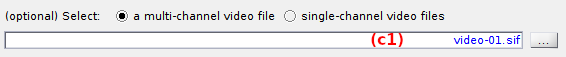
To import a multi-channel video or image, press and select the corresponding file.

Once the import is completed, the multi-channel video file name is shown in (c1).

Import of single-channel videos

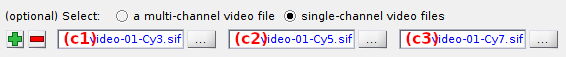
To import single-channel videos or images, set, first, the appropriate number of channels using the Plus or Minus button to add or remove channels, respectively. The channel configuration is automatically updated in tab Channels.

After the number of video channels is correctly set, import each single-channel video by pressing the appropriate button and selecting the corresponding file.

Once the import is completed, single-channel video file names are shown in (c1)-(c3).

Coordinates file

Single molecule coordinates are used to recalculate intensity time traces when the molecule position is modified and in a specific background calculation. If no coordinates are available, intensities will not be recalculated and only manual background setting will be allowed.

To import a coordinates file, press and select the proper file. After import, the file name is displayed in (a).

The coordinates file contains the x- and y- pixel positions of each single molecule in each emission channel. It must be structure following certain rules:

molecules must be written in rows
x- and y-coordinates must be organized in columns

Coordinates are read using the import settings that can be modified by pressing Import options .

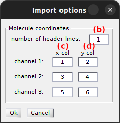
The number of file header lines is set in (b) and channel-specific x- and y-coordinates are read from columns set in (c) and (d) respectively. Import settings are saved only after pressing .

Correction factor files

Gamma factors account for differences in emission detection efficiencies and quantum yields between donor and acceptor emitters, whereas beta factors account for differences in extinction coefficients and excitation intensities.

Gamma factors are used in FRET and stoichiometry calculations, whereas beta factors are used in stoichiometry calculations only; see Correct ratio values for more information.

Correction factors are usually calculated or set in panel Factor corrections, but can also be imported from one or several files along with the trajectories.

To import gamma and/or beta factors, press the corresponding button and select the proper file(s). The imported file names are then displayed in (a) and/or (b) respectively.

Gamma and beta factor files are structured as described in .gam files and .bet files respectively.

If several files are selected, gamma and/or beta factors will be concatenated row-wise.

Channels

Use this tab to configure the emission channels.

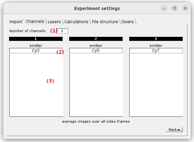
If not already done in the Import tab when defining the single-channel video files, the number of emission channels in your experiment must be set in (1). Upon modification, the tab interface is automatically adjusted.

Each emission channel is associated to a particular emitter and must be labelled accordingly in (2). These labels are later used to identify the corresponding trajectories.

When a video was imported along with the trajectories, channel plots in (3) show the portion of the average image that correspond to each emission channels; see Video-based project for more details. Otherwise, they are left blank.

default: 2 channels labelled chan [c], with [c] the channel index.

Lasers

Use this tab to configure the illumination setup.

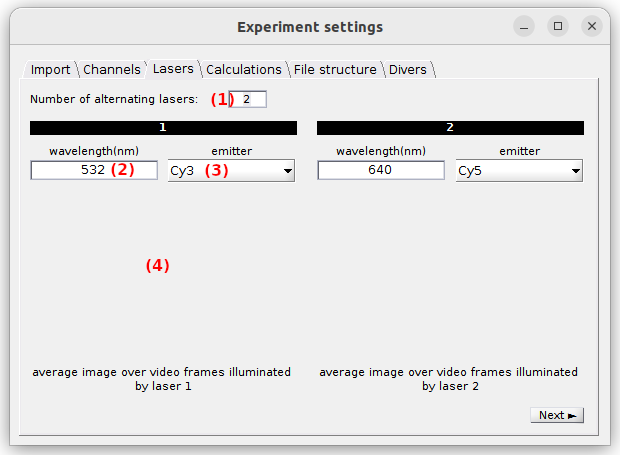
The number of alternated lasers with different wavelengths used in the experiment is set in (1). For continuous-wavelength excitation, it must be set to 1. Upon modification, the tab’s interface is automatically adjusted.

Selective emitter excitation and laser wavelength must be defined for each laser by selecting the proper emitter in (3) and typing the the wavelength in nanometers in (2). These two parameters are used to label data and sort emitters according to the red-shift of there absorption spectra, which is necessary in FRET and stoichiometry calculations; see Calculations for more details.

If a video was imported along with the trajectories, plots in (4) show the average images of the video frames recorded upon illumination of each laser, lasers being numbered following the chronological order in the video; see Video-based project for more details.

default: one laser, wavelength: 532 nm, emitter: channel 1

Calculations

Use this panel to define the FRET and stoichiometry ratios to be calculated and plotted.

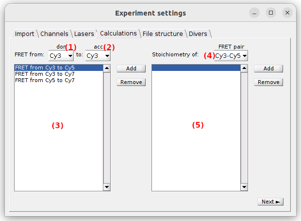
The FRET and Stoichiometry ratios are calculated according to FRET calculations and Stoichiometry calculations, respectively.

To activate the FRET calculation for a FRET pair in particular, selective laser excitation of the donor must be present in the experiment. In this case, select the donor and acceptor channel labels in list (1) and (2), respectively, and press Add . All FRET calculations are listed in (3) and can be removed any time by pressing Remove .

To activate the stoichiometry calculation for a FRET pair in particular, the FRET pair must be listed in (3) and selective laser excitation of the acceptor must be present in the experiment. In this case, select the desired FRET pair in (4) and press Add . All stoichiometry calculations are listed in (5) and can be removed any time by pressing Remove .

default: no calculations

FRET calculations

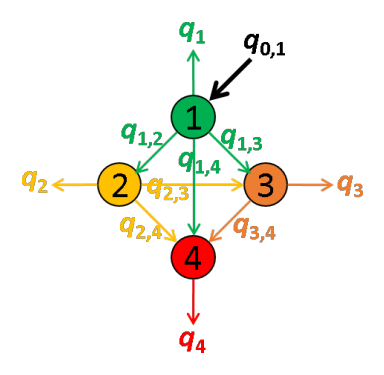
In a network composed of several emitters, quantities of energy absorbed by each of the emitters can be emitted as light or transferred via FRET to other emitters providing a non-negligible overlap of the donor emission spectrum with the absorption spectra of the acceptors.

These energy movements can be represented on a scheme where:

emitters are numbered according to the red shift of the absorption spectrum
the energy quantity absorbed by emitter i exclusively is noted q_0,i,
the quantity of energy emitted by emitter i is noted q_i,
the energy quantity transferred by FRET from emitter i to emitter j is noted q_i,j.

For example, the energy movements in a FRET-pair network composed of four emitters with different absorption and emission properties are summarized in the following scheme.

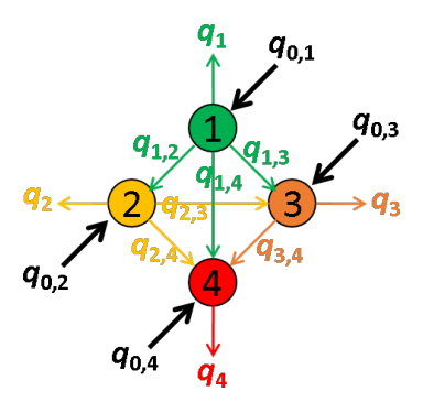
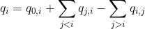
In an ideal system that includes radiative processes and energy transfers only, the law of conservation of energy supposed that:

$q_{i}=q_{0,i}+\sum_{j<i}q_{j,i}-\sum_{j>i}q_{i,j}$

The energy quantity q_i is comparable to the intensity detected in emission channel of emitter i and corrected from background and cross-talks. Thus, q_i values are measured during the experiment.

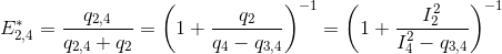
The apparent efficiency E*_D,A of an energy transfer from a donor D to an acceptor A is calculated as:

$E_{D,A}^{*}=\frac{q_{D,A}}{q_{D}+q_{D,A}}$

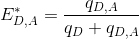
To obtain the probability of energy transfer E_D,A, which is inversely proportional to the distance r between the two dyes, E*_D,A must later be corrected by considering (1) the different quantities of non-radiative energy lost during the process by both emitters D and A as well as (2) the different detection efficiencies of photons emitted by emitters D and A; see Correct ratio values for more information.

The energy quantity q_i,j is calculated from intensities measured upon different laser illuminations, starting with specific excitation of the most red-shifted donor. For the limiting case where the most red-shifted donor transfers energy to multiple acceptors, FRET efficiencies can not be analytically calculated.

Translated in a four-emitter network, the most red-shifted donor is the emitter 3, which can transfer energy to emitter 4 only. This comes down to a simple two-emitter network where energy movements can be depicted as in the following scheme.

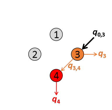
Using the law of conservation of energy and the definition of the apparent FRET efficiency of the donor-acceptor pair 3- 4, we can readily calculate E*_3,4 from measured intensities such as:

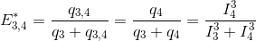
$E_{3,4}^*=\frac{q_{3,4}}{q_3+q_{3,4}}=\frac{q_4}{q_3+q_4}=\frac{I_4^3}{I_3^3+I_4^3}$

The next most red-shifted donor is the emitter 2, which can transfer energy to emitters 3 and 4. This comes down to a three-emitter network where energy movements can be depicted as in the following scheme.

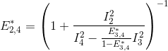
Using the law of conservation of energy and the definition of the apparent FRET efficiencies of the donor-acceptor pairs 2- 3 and 2-4, we can express E*_2,3 and E*_2,4 in function of measured intensities and the quantity q_3,4 such as:

$E_{2,3}^*=\frac{q_{2,3}}{q_{2,3}+q_2}=\left (1+\frac{q_2}{q_3+q_{3,4}}\right )^{-1} = \left ( 1+\frac{I_2^2}{I_3^2+q_{3,4}}\right )^{-1}$
$E_{2,4}^*=\frac{q_{2,4}}{q_{2,4}+q_2}=\left (1+\frac{q_2}{q_4-q_{3,4}}\right )^{-1} = \left ( 1+\frac{I_2^2}{I_4^2-q_{3,4}}\right )^{-1}$

According to the definition of the apparent FRET efficiency, q_3,4 can be expressed in function of measured intensities and the known E*_3,4, such as:

$q_{3,4}=\frac{E_{3,4}^*}{1-E_{3,4}^*}I_3^2$

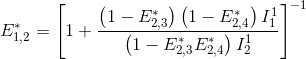
Put together, these equations allow to calculate E*_2,3 and E*_2,4 in function of measured intensities and the known E*_3,4, such as:

$E_{2,3}^*= \left ( 1+\frac{I_2^2}{I_3^2+\frac{E_{3,4}^*}{1-E_{3,4}^*}I_3^2}\right )^{-1}=\left [ 1+\frac{I_2^2\left( 1-E_{3,4}^*\right )}{I_3^2}\right ]^{-1}$
$E_{2,4}^*= \left ( 1+\frac{I_2^2}{I_4^2-\frac{E_{3,4}^*}{1-E_{3,4}^*}I_3^2}\right )^{-1}$

The next most red-shifted donor is the emitter 1, which can transfer energy to emitters 1, 3 and 4. Energy movements can be depicted as in the following scheme:

FRET efficiencies for the FRET pairs 1-2, 1-3 and 1-4 are determined using the same deductive path as presented above, giving:

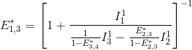
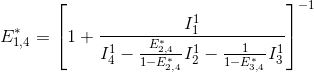
This demonstration can be generalized to a K-emitter network with the apparent FRET efficiency E*_D,A – of a donor-acceptor pair D-A with A>D – being calculated from intensities detected upon excitation of emitter D and apparent FRET efficiencies obtained from more red-shifted FRET-pairs, such as:

$E_{D,A}^*= \left \{ 1+\frac{I_{D,em}^{D,ex}}{I_{A,em}^{D,ex} \left [1+\sum_{i>A}\left (\frac{E_{A,i}^*}{1-E_{A,i}^*}\right )\right ] -\sum_{D<i<A}\left( \frac{E_{i,A}^*}{1-E_{i,A}^*}I_{i,em}^{D,ex}\right )} \right \}^{-1}$

with I_k,em^k’,ex,*** the intensity collected in channel specific to emitter k, upon laser illumination that specifically excites emitter k’, and after background and cross-talk corrections.

To know more about how multi-color apparent FRET data are calculated, please refer to the respective functions in the source code:

MASH-FRET/source/mod-trace-processing/FRET/buildFretexpr.m
MASH-FRET/source/mod-trace-processing/FRET/calcFRET.m

Stoichiometry calculations

The stoichiometry of an emitter is usually used to estimate the ratio of different emitters attached to the single molecule under observation.

The apparent stoichiometry S*_D,A for a FRET pair composed of donor emitter D and an acceptor emitter A, specifically excited by the respective illuminations D_ex and A_ex in a labelling scheme consisting of K emitters, is calculated as:

$S_{D,A}^{*} = \frac{\sum_{k}\left (I_{k,em}^{D,ex} \right )}{\sum_{k}\left( I_{k,em}^{D,ex} + I_{k,em}^{A,ex} \right ) }$

with I_k,em^k’,ex,*** the intensity collected in channel specific to emitter k, upon laser illumination that specifically excites emitter k’, and after background and cross-talk corrections.

To obtain the stoichiometry S_D,A, which correspond to the ratio of different emitters attached to the single molecule under observation, S*_D,A must later be corrected by considering the differences for emitters D and A in: (1) quantities of non-radiative energy lost during the process by the emitters, (2) camera detection efficiencies of emitter photons, (3) quantities of energy released by the emitter-specific illuminations, (4) quantities of energy absorbed by the emitters; see Correct ratio values for more information.

A stoichiometry S_D,A = 0.5 means that half of the total number of D and A emitters attached to the molecule are D emitters.

To know more about how multi-color Stoichiometry is calculated, please refer to the respective functions in the source code:

MASH-FRET/source/mod-trace-processing/FRET/buildSexpr.m
MASH-FRET/source/mod-trace-processing/FRET/calcS.m

File structure

Use this tab to define the structure of trajectory files.

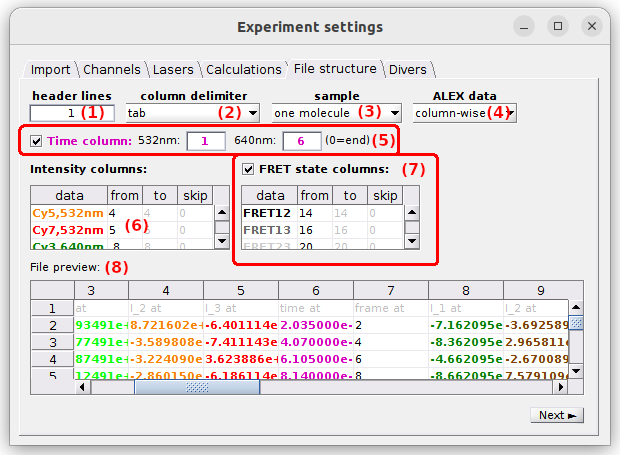
Set parameters parameters (1) to (7) to define the structure of the trajectory files. Use the File preview in (8) to verify the proper reading of file columns and trajectory data when adjusting parameters.

(1) Header lines
(2) Column delimiter
(3) Molecule sample
(4) ALEX data organization
(5) Time data
(6) Intensity data
(7) FRET state sequence data
(8) File preview

The structure define on the example above is used to import Processed trace files of a 3-channel and 2-laser experiment. The other trajectory file structure used by MASH is the one of Trace files from video and would correspond to the following settings:

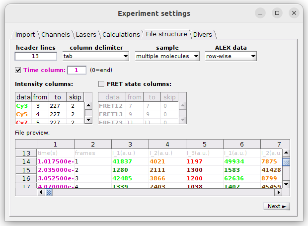
Header lines

The number of header lines is the number of lines on top of the file that do not contain any intensity data. Header lines are represented with a gray-colored font in the File preview.

Column delimiter

Column delimiters are characters written in the file that separate column data. Supported delimiters are:

blanks (tab,spaces): both tab and space characters
tab: tab character (in most ASCII files exported from MASH)
,: comma character
;: semi-column character
space: space character

You can ensure a proper column separation by using the File preview.

Note : In later versions, the supported file structures will be extended with a custom delimiter and the .json format.

Molecule sample

The molecule sample indicates whether the file contains data of one or multiple single molecules:

one molecule: data are imported for only one molecule and Intensity data and FRET state sequence data are written in single columns (labelled: from),
multiple molecules: data are imported for multiple molecules and Intensity data and FRET state sequence data are written in column ranges (labelled: from, to, skip), where the number of columns scales with the number of molecules.

You can ensure a proper reading of molecule-specific data by using the File preview.

ALEX data organization

Data from experiments that use alternating lasers can be organized in two ways:

row-wise: Data are written as they are recorded, meaning that each row in the file is a recording step. In this case, data recorded under a specific laser illumination are written every nL rows, with nL the number of lasers alternated in the experiment.
column-wise: Specific data recorded under specific laser illuminations are written in specific file columns.

Data in the File preview are colored following the Plot colors to ensure a proper reading of laser-specific data.

Time data

This interface defines the organization of time data in the file and depends on the ALEX data organization:

row-wise: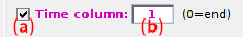

If the files contain time data, activate the option in (a) and set in (b) the file column where time data are located.
column-wise:

If the files contain time data, activate the option in (a) and set in (b)-(c) the file column where laser-specific time data are located.

If trajectories are imported without video, the Video sampling time is deduced from the time data and is automatically updated in tab Divers.

Time data are colored in pink in the File preview to ensure a proper reading of time columns.

Intensity data

This table defines the file columns where intensity data are written and depends on the Molecule sample and ALEX data organization.

The first table column data lists the data for which the file columns have to be defined. They are colored according to the Plot colors and named after the channel labels [em] and the laser wavelengths [wl], depending on the ALEX data organization:

[em] for a row-wise organization
[em]at[wl]nm for a column-wise organization

Intensity columns in the files are then defined in table columns:

from: the only column where data are written if the Molecule sample is set to one molecule, or the first column of the range if it is set to multiple molecule,
to: (only for multiple molecule) last column of the range,
skip: (only for multiple molecule) the number of columns to skip to find the data of the next molecule.

Data in the File preview are also colored according to the Plot colors to ensure a proper reading of intensity columns.

FRET state sequence data

This interface defines the import of FRET state data.

Imported FRET state trajectories will be shown in Trace processing and used in Transition analysis and Histogram analysis modules. If imported trajectories are pocessed in module Trace processing, state sequences will be overwritten by the newly calculated ones.

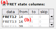
To import FRET state trajectories, activate the option (a) and set the file columns in table (b).

Table (b) defines the file columns where FRET state data are written and depends on the Molecule sample. The first table column data lists the FRET pairs for which the file columns have to be defined. They are colored according to the Plot colors and named after the donor and acceptor channel indexes. FRET state columns in the files are then defined in table columns:

from: the only column where data are written if the Molecule sample is set to one molecule, or the first column of the range if it is set to multiple molecule,
to: (only for multiple molecule) last column of the range,
skip: (only for multiple molecule) the number of columns to skip to find the data of the next molecule.

Data in the File preview are also colored according to the Plot colors to ensure a proper reading of FRET state columns.

Note: After import, the first molecule in the sample is automatically processed in module Trace processing and state sequences are overwritten by the newly calculated ones; this will be corrected in later versions. However, the state sequences used in Transition analysis and Histogram analysis are not affected as long as all molecule data are not processed at once in Trace processing; see Process all molecules data.

File preview

The file preview shows the content of the first trajectory file using the current define structure. The file content is color-coded, where Header lines are grayed out, Time data are colored in pink, and Intensity data and FRET state sequence data are color-coded using the Plot colors.

It can be used to verify the proper reading of file columns and trajectory data when adjusting parameters (1)-(7).

Divers

Use this tab to define the project’s title, optional parameters, the video sampling time and plot colors.

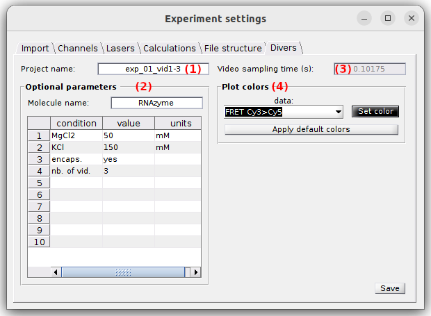
(1) Project’s title
(2) Optional parameters
(3) Video sampling time
(4) Plot colors

Project’s title

The title is the name appearing in the project list. It is defined in (1). Leaving (1) empty will give the title “Project” to your project.

default: trajectories

Optional parameters

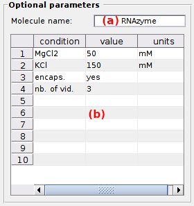
Optional parameters include the name of the investigated molecule, set in (a), and the experimental conditions set in (b).

Experimental conditions can be added, modified and removed by simply editing the condition’s name, value and units in the corresponding column of table (b).

Optional parameters solely act as project “tags” saved with the MASH project file and exported in Processing parameter files.

default: [Mg2+] in mM (magnesium molar concentration) and [K+] in mM (potassium molar concentration).

Video sampling time

The video sampling time is shown in seconds in (3). In the case the sampling time was successfully read from either the trajectory files or the video file, this property is read-only. If not, the sampling time must be set manually.

default: 1 second

Plot colors

Use this panel to define the colors used to plot and identify the time traces.

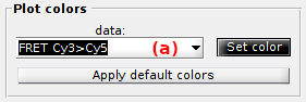
To set the RGB color of a specific trace, select the data in list (a) and press Set color to open the color picker.

To use a predefined set of colors adapted to the experiment design, press Apply default colors .

default: from green to red for intensities, shades of black for FRET ratios and shades of blue for stoichiometry ratios.

<< PREVIOUS: Video-based project NEXT: Histogram-based project >>