![]()
Molecules
Molecules is the second panel of module Simulation.
Access the panel content by pressing
 .
The panel closes automatically after other panels open or after pressing
.
The panel closes automatically after other panels open or after pressing
 .
.
Use this panel to define the molecule sample in terms of size, positions and of molecule and dye properties.
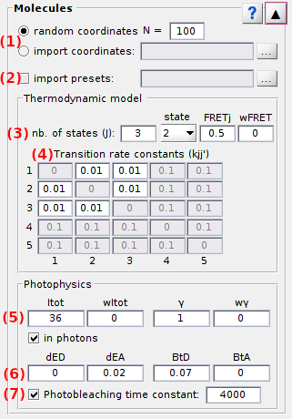
Panel components
- Molecule positions
- Pre-set parameters
- State configuration
- Transition rates
- Donor emission
- Cross-talks
- Photobleaching
Molecule positions
Use this interface to define the number and positions of molecules in the simulated field of view.
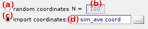
The number of single molecules to simulate, noted N, is shown in (b).
Molecule positions in the simulated field of view can be aquired in two was:
- Randomly generated by activating (a),
- Imported from an external ASCII file by activating (c).
Random positions
To generate random molecule positions, activate the option (a) and type in (b) the number of single molecules N to be simulated.
Import positions
To import molecule positions from an external ASCII file, activate the option (c) and select the appropriate file in the browser. After successful import, the file name is displayed in (d) and the number of molecule derived from the file is shown in (b).
For the positions to be correctly imported, certain rules must be followed:
- the file must be structured in two or four columns, with x- and y-positions written in odd and even columns respectively.
- if the file contains left- or right-channel coordinates only, coordinates in the other channel are automatically calculated by adding or subtracting one channel width to x-positions.
- imported coordinates can me dismissed by reactivating the option (a)
Coordinates can also be imported from a pre-set parameter file; see Pre-set parameters for more details.
default: N = 100 molecules with randomly generated positions.
Pre-set parameters
Use this interface to import pre-defined parameters for individual molecules from an external MATLAB binary file (.mat).
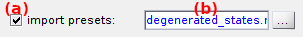
Pre-set parameters can be imported from an external .mat file by activating (a). In that case:
- the file must contain a MATLAB structure with at least one of the following fields:
| field name | description | data type |
|---|---|---|
FRET |
FRETj values and deviations wFRETj for a J-state model; see State configuration for more details about the meaning of these values | J-by-2-by-Ndouble |
trans_rates |
transition rate matrix restricted to 2 states kjj’ | J-by-J-by-N double |
trans_prob |
transition probability matrix wjj’ being in state j (normalized row-wise) | J-by-J-by-N double |
ini_prob |
initial state probabilities | N-by-J double |
gamma |
γ factors and deviations wγ; see Donor emission for more details about the meaning of these values | N-by-2 double |
tot_intensity |
intensities Itot,em and deviations wItot,em; see Donor emission for more details about the meaning of these values | N-by-2 double |
coordinates |
x- and y- molecule coordinates in donor and/or acceptor channel | N-by-2 or -4 double |
psf_width |
PSF standard deviations wdet,D and/or wdet,A in donor and/or acceptor channel respectively | N-by-1 or -2 double |
- if parameter
trans_probis absent, uniform transition probabilities are defined - if parameters
ini_probis absent, initial state probabilities are calculated from the unrestricted transition rate matrix - if parameter
coordinatescontains coordinates in only one channel, x-positions are automatically translated to obtain coordinates in the other channel. - if parameter
psf_widthis of dimension N-by-1, PSF widths are applied to both channels. - loaded pre-sets can me removed by deactivating (a)
After successful import:
- imported file name is displayed in (b)
- the field used to edit the number of molecules in Molecule positions will be locked as it is set by any preset parameter
- the field used to edit the number of states in
State configuration will be locked if
FRETortrans_ratesare defined - the fields used to edit the
FRETj and
wFRETj values in
State configuration will be locked if
FRETis defined - the fields used to edit the
Transition rates will be locked if
trans_ratesis defined - the fields used to edit the
Itot,em and
wItot,em values in
Donor emission will be locked if
tot_intensityis defined - the fields used to edit the
γ and
wγ values in
Donor emission will be locked if
gammais defined - the fields used to edit the
wdet,D and
wdet,A values in
Point spread functions will be locked if
psf_widthis defined
Fields will be rendered editable when removing the pre-set file.
A *.m template file is provided with the source code at:
MASH-FRET/tools/createSimPrm.m
default: no parameter file is loaded, all parameters are set via the GUI.
State configuration
Use this interface to define the number of states and corresponding FRET values.
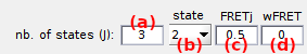
The state configuration is described by a number
J of states set in (a), and the corresponding
FRETj values set in (c) after selecting state [j] in list (b), with [j] the state index.
If needed, sample heterogeneity can be introduce by attributing a strictly positive deviation wFRETj (d) to the FRETj value. In this case, a random FRET value is drawn for each molecule, using a Gaussian distribution with mean FRETj and standard deviation wFRETj.
default:
Transition rates
Use this interface to define the rate coefficients that govern state transitions, noted kjj’.
Transition rates are given in second-1 and are organized in a matrix, where the cell (row j, column j’) concerns the unidirectional transition from state j to state j’.
A rate set to zero defines a forbidden transition.
Heterogeneous transition kinetics are characterized by multiple rate coefficients and can be simulated by using degenerated states, i.e., using states with same FRETj value but different transition rate coefficients. For an example, please refer to the literature1.
default: 0.1 second-1.
Note: For more practicability, the transition rate matrix is limited to five states. To simulate a system with more than five states, please refer to Simulate more than five states
References
- S. Schmid, T. Hugel, Efficient use of single molecule time traces to resolve kinetic rates, models and uncertainties, J. Chem. Phys. 2017, DOI: 10.1063/1.5006604
Donor emission
Sets the donor emission intensity in absence of acceptor, noted Itot,em.
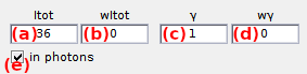
Intensity Itot,em is set in (a) and is given in units defined in Intensity units.
If needed, sample heterogeneity can be introduced by attributing a strictly positive deviation wItot,em (b). In this case, a random intensity value is drawn for each molecule, using a Gaussian distribution with mean Itot,em and standard deviation wItot,em.
Differences in donor and acceptor quantum yields and detection efficiencies can be modulated by setting the factor γ in (c). Donor emission is affected according to the relation:
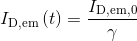
with ID,em,0 the original donor fluorescence intensity in presence of acceptor, and ID,em the gamma-modified version.
Thus, introducing a gamma factor lower or higher than 1 place the donor intensity on a different scale than acceptor intensity.
Similarly to the intensity, sample heterogeneity in gamma factor can be introduced by setting a strictly positive deviation wγ in (d).
Intensity units
Intensity units of Itot,em and wItot,em can be set in photon counts (pc) or camera offset-free image counts (ic) when the option in (e) is activated or inactivated respectively. This choice also affects the units of background intensities set in Background.
Photon counts μpc and camera offset-free image counts μic are linked by the relation:
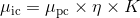
with camera characteristics η and K, the detection efficiency and overall gain respectively.
Camera offset-free image counts are used here because experimental Itot,em value can be obtained by averaging the sum of donor and acceptor intensity-time traces in Trace processing after background correction, which includes subtraction of camera offset.
If one of the characteristics is not defined within the chosen camera noise model, the following default values are used:
See Camera SNR characteristics for more information.
Only photon counts μpc are registered in memory. Image counts are recalculated every time another camera noise model with different η and K is selected.
default:
Cross-talks
Use this interface to set the direct excitation and bleedthrough coefficients.
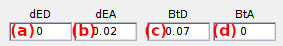
Cross-talks bias the measured fluorescence intensities because of instrumental imperfections.
The donor and acceptor direct excitation coefficients dED and dEA are the fractions of signal collected when illuminated by the pair’s excitation wavelength. They can be set in (a) and (b) respectively. Here, setting dED is senseless as simulations are limited to continuous- (donor-) wavelength excitation.
The donor and acceptor bleedthrough coefficients btD and btA are the fractions of signal leaking in the pair’s channel. They can be set in (c) and (d) respectively.
default: default coefficients are based on our experimental setup:
Photobleaching
Defines the time spent before photochemical destruction of the donor fluorophore.
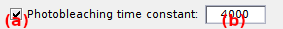
Photochemical destruction of the donor, i.e., photobleaching, can be activated by activating the option in (a). In that case, intensity-time traces are interrupted at random photobleaching time by a sudden and irreversible extinction of donor emission.
Photobleaching times are randomly drawn for each molecule from an exponential distribution with a decay constant set by (b).
default: no photobleaching, the observation time is set by video length L.