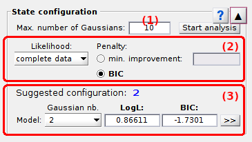
State configuration

State configuration is the second panel of module Histograms analysis. Access the panel content by pressing Bottom arrow . The panel closes automatically after other panels open or after pressing Top arrow .

Use this panel to determine the optimum number of histogram peaks.

Panel components

Maximum number of Gaussians
Model penalty
Inferred models

Maximum number of Gaussians

Defines the maximum model complexity to consider for model fitting, i.e., the maximum number of Gaussian in the Gaussian mixture models to infer; see Determine the most sufficient state configuration in Histogram analysis worklow for more information about state configuration analysis.

The maximum number of Gaussian in the model is the only parameter necessary to infer models.

Press Start analysis to start model inference.

default: 10

Model penalty

Use this interface to define model overfitting penalty.

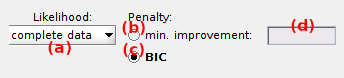
The goodness of the gaussian mixture fit is evaluated by the likelihood of the model. The likelihood can be calculated in two manners listed in (a):

complete data where each bin is associated to one and only Gaussian,
incomplete data where bins have a non-null probability to belong to each Gaussian (subject to overestimation of model complexity).’

In both cases, the likelihood inevitably increases with the fit model compexity. To prevent overfitting, the likelihood can be penalized in two ways:

Minimum improvement in likelihood, by activating the option in (b)
Bayesian information criterion (BIC), by activating the option in (c)

The overfitting penalty can be modified before or after inferring the different models, i.e., before or after pressing Start analysis .

Minimum improvement in likelihood

With this penalty, a certain improvement in the model log-likelihood is expected when adding a new component to the model. The improvement is expressed as a multiplication factor that can be set in (d). For instance, set a penalty of 1.2 for an improvement of 20% in the log-likelihood, or of 10^0.2 in the likelihood.

The most sufficient model is the least complex model for which adding a component does not fulfill this requirement.

Bayesian information criterion

The BIC is used to rank models according to their sufficiency, with the most sufficient model having the lowest BIC.

The BIC is similar to a penalized likelihood and it is expressed such as:

$BIC\left (V \right ) = p\left (V \right ) \times \log ( M_{\textup{total}} ) - 2 \times \log \left [ likelihood\left (V \right ) \right ]$

with p the number of parameters necessary to describe the model with V components and M_total the total number of counts in the histogram.

The number of parameters necessary to describe the model includes the number of Gaussian means p_means, standard deviations p_widths and relative weights p_weights, and is calculated such as:

$p\left ( V\right ) = p_{\textup{means}} + p_{\textup{widths}} + p_{\textup{weights}} = 3V - 1$

Inferred models

Use this interface to visualize the results of state configuration analysis.

The number of components in the most sufficient model according to the Model penalty is shown in (a) and the corresponding gaussian mixture can be visualized in the Top axes.

Other inferred models can be visualized by selecting the corresponding number of components in the list (b). In this case, the log-likelihood and BIC of the selected model are respectively displayed in (c) and (d).

The parameters of any model can be imported in Thresholding or Gaussian fitting as starting guess for state population analysis, by pressing .