![]()
Use Trace manager
The trace manager gives an overview of all single molecules in the project and allows to assemble a molecule selection as well as to give molecules specific tags.
It is accessed by pressing
 in the
Sample management panel of module Trace processing.
in the
Sample management panel of module Trace processing.
Trace manager is used to sort molecules into sub-groups and/or exclude irrelevant traces from the set. It is composed of three modules:
Overview Automatic sorting Video view
Automatic sorting
Automatic sorting is used to tag groups of molecules based on specific data criteria.
Tags are eventually applied to individual molecules after pressing
 .
.
Automatic sorting is divided into three panels (1-3) and one visualization area (4-5).

Interface components
Data
Use this panel to define the data to be sorted and displayed.

Auto-sorting works with the molecule selection assembled in Overview. The 1D- or 2D- histogram used in Auto-sorting will be recalculated each time the molecule selection changes.
Data available for 1D- or 2D-sorting are listed in menu (a) (x-axis) and (f) (y-axis) and include:
[E] at [W]nmfor intensity data, with[E]the emitter and[W]the laser wavelengthtotal [E] (at [W]nm)for intensity-time traces of emitter[E]in absence of any acceptor and upon emitter-specific excitation wavelength[W]FRET [D]>[A]for FRET data, with[D]and[A]the donor and acceptor emitters respectivelyS [D]>[A]for stoichiometry data associated to the FRET pair where[D]and[A]are the donor and acceptor emitters respectivelyFRET [D]>[A]-S [D]>[A]for 2D FRET-Stoichiometry data
For 1D-sorting, menu (f) must be set to none.
Data are sorted into bins defined by (c) (lowest limit), (d) (highest limit) and (e) (bin size) for the x-axis, and by (h), (i) and (j) for the y-axis.
Data can be counted as one count per molecule in the 2D-histogram by activation option (l).
2D-histograms can be displayed with Gaussian filtering by activating option (k).
Molecule sorting can be performed on full-length data-time traces or state trajectories, but also on different descriptive statistics or state data. The type of data sets can be selected in menu (b) (x-axis) and (g) (y-axis) and include:
original time traces (frame-wise)for full-length data-time tracesstate trajectories (frame-wise)for full-length data state trajectoriesmeans (molecule-wise)for the means of the data-time tracesminima (molecule-wise)for the maxima of the data-time tracesmaxima (molecule-wise)for the minima of the data-time tracesmedians (molecule-wise)for the medians of the data-time tracesSNR (molecule-wise)for the signal-to-noise ratio of the data-time traces \(data(t)\), calculated from mean value \(\langle data\rangle\) and trajectory length \(L\) with: \(SNR=\frac{\langle data \rangle }{\sqrt{\frac{1}{L-1}\sum_t{data(t)-\langle data\rangle}}}\)bleaching cutoff (molecule-wise)for the time point at which photobleaching of emitter[E]was detectednb. of states (molecule-wise)for the number of states in state trajectoriesnb. of transitions (molecule-wise)for the number of state transitions in state trajectoriesmean dwell time (molecule-wise)for the average state dwell times of the state trajectoriesstate values (state-wise)for the individual state values in the state trajectoriesstate dwell times (state-wise)for the individual state dwell times in the state trajectoriesstate lifetimes (state-wise)for the individual state lifetimes \(\tau\) estimated from transition numbers \(N_{ij}\) and trajectory length \(L\) with: \(\tau_i=\frac{L}{\sum_{j \neq i} N_{ij}}\)
For 2D-sorting, x-axis and y-axis data sets must occur on the same scale (frame-wise, molecule-wise or state-wise).
To use the options state trajectories, nb. of states, nb. of transitions, mean dwell time, state values or state dwell times, all the molecules of the selection must have the corresponding data-time trace discretized.
If some state trajectories are missing, a warning pops up.

To perform 2D-sorting on the transition density plot, x-axis and y-axis data must be identical and the state values set must be chosen for both.
Resulting 1D- or 2D-data histogram is plotted in Histogram plot and can be exported to a .txt file by pressing 
Range
Use this interface to configure sorting settings
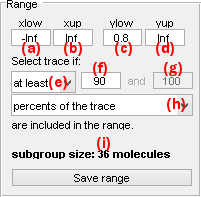
The data set defined in panel Data is sorted according to a specific value range. The range is defined by a minimum value set in (a) or (c) and a maximum value set in (b) or (d) for the x- or y-axis respectively. Range bounds can also be defined by simply clicking on the Histogram plot.
The range is represented on the Histogram plot with out-of-ranges values being covered by a transparent black mask.
If the data set is scaled frame-wise (data original time traces or state trajectories), the confidence level for inclusion in the range must be defined.
The confidence level can be set as:
at leastwith the minimum confidence level set in (f)at mostwith the maximum confidence level set in (f)betweenwith the minimum and maximum confidence levels set in (f) and (g) respectively
The confidence levels in (f) and (g) can be expressed in trace percentage or in number of data points per trace by selecting the respective options percents of the trace or data points in menu (h).
The resulting number of molecule included in the current range is displayed in (i).
To define a subgroup affiliation for the molecules included in the current range, settings must be saved by pressing
 .
Additionally, when saved, range settings can be accessed any time in the subgroup list of panel
Tags.
.
Additionally, when saved, range settings can be accessed any time in the subgroup list of panel
Tags.
Tags
Use this interface to define subgroup affiliations (tags).

Ranges saved in panel
Range are listed in (a) and can be deleted from memory by pressing
 .
.
To define a subgroup affiliation for the molecules included in range selected in list (a), choose a tag in menu (b) and press
 .
All tags assigned to the selected subgroup are listed in (c) and can be removed one by one by pressing
.
All tags assigned to the selected subgroup are listed in (c) and can be removed one by one by pressing
 .
.
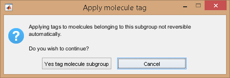
Molecule tags are eventually applied to individual molecules after pressing
; as the operation can not be reversed, a confirmation warning pops up.
Histogram plot
Use this interface to visualize the data distribution and define the data range by clicking.
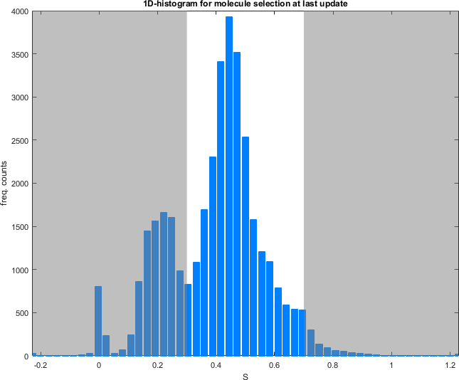
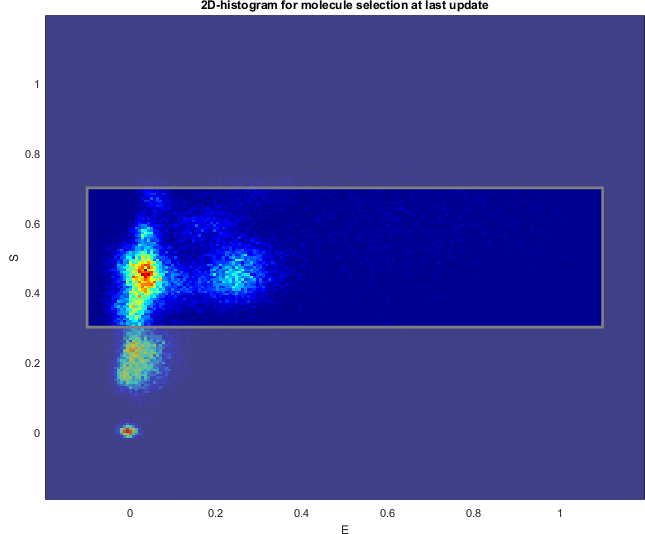
Data is distributed into a 1D- or 2D-histogram built with settings defined in Data.
Ranges defined in Range or defined by clicking on the plot, are highlighted in white for 1D-histograms and within a gray rectangle for 2D-histograms. Out-of-range data covered with a transparent black mask.
Concatenated trace plot
Use this interface to visualize the time-traces affiliated to the current molecule subgroup.
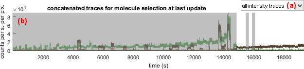
The concatenated trace plot shows time-traces of the molecule selection at last update in panel Overall plots.
Concatenated trace plot allows to visualize which time traces are included or excluded from the current subgroup. Included time traces are highlighted with a white background and excluded time traces are covered with a transparent black mask.
Data available for concatenated trace plot are listed in menu (a) and include:
[E] at [W]nmfor intensity-time traces, with[E]the emitter and[W]the laser wavelengthtotal [E] (at [W]nm)for intensity-time traces of emitter[E]in absence of any acceptor and upon emitter-specific excitation wavelength[W]FRET [D]>[A]for FRET-time traces, with[D]and[A]the donor and acceptor emitters respectivelyS [D]>[A]for stoichiometry data associated to the FRET pair where[D]and[A]are the donor and acceptor emitters respectively